
On Friday, the GCDI Digital Fellows hosted a workshop on how to use online libraries and programming languages for text analysis purposes. The session revolved around Python and its Natural Language Tool Kit (NLTK), an inbuilt platform that specifically works with human language data. NLTK allows the conversion of texts, such as books, essays and documents, into digitally consumable data, which implies a transformation of qualitative contents into quantitative, and therefore decomposable and countable, items. The workshop did not require prior experience with NLTK and resulted in an extremely effective session.
I thought of different ways of summarising what was covered during the seminar in a way that other people would find useful and decided to write a step-by-step guide that incapsulates the main aspects discussed and some additional pieces of information that can be helpful when approaching Python and Jupyter Notebook from scratch.
Required downloads/installations
- A Text Editor (aka where the user writes their code) of your choice, I opted for Visual Studio Code, alternatively Notepad would do – FYI: Google Docs & Microsoft Word will not work since they are not text editors, but word processors;
- Anaconda;
- Git for Windows , for Windows users only. This is optional, but I would still recommend it.
About Python
- There is extensive documentation available, including the official Beginner’s Guides.
- It is an interpreted language, hence it does what the user tells it to.
- It is object-oriented; mostly Python has ‘classes’ of objects, and almost everything is an object.
- Python is designed to be readable.
Jupyter Notebook
Jupyter Notebook is structured data that represents the user’s code, metadata, content, and outputs. When saved to disk, the notebook uses the extension .ipynb, and uses a JSON structure. Jupyter Notebook and its interface extend the notebook beyond code to visualisation, multimedia, collaboration, and more. In addition to running codes, it stores code and output, together with markdown notes, in an editable document called a notebook. When saving it, this is sent from the user’s browser to the notebook server which, in turn, saves it on disk as a JSON file with a .ipynb extension.
Remember: do save each new file/notebook with a name, otherwise it will be saved as “unnamed file”. You can type in your search bar Jupyter and see if it is already installed on your computer, otherwise you can click > Home Page – Select or create a notebook
When ready, you can try the below steps in your Jupyter Notebook and see if they produce the expected result/s. To comment in Jupyter you can use the dropdown menu selecting “markdown” instead of “code”. Alternatively, you can use either 1 or 2 # signs.
In Jupyter every line can be a code, or a comment, and each line can be run independently – also, lines can be amended and rerun.
To start type these commands in your Jupyter Notebook (commands are marked by a bullet point and comments follow in Italic):
- import nltk
- nltk stands for natural language tool kit
- from nltk.book import *
- the star means “import everything”
- text1[:20]
- for your reference: text1 is Moby Dick
- this command prompts the first 20 items of the text
- text1.concordance(‘whale’)
- Concordance is a method that shows the first 25 occurrences of the word whale together with some words before and after – so the user can understand the context – this method is not case sensitive
Before proceeding, let’s briefly look at matplotlib.
What is matplotlib inline in python
IPython provides a collection of several predefined functions called magic functions, which can be used and called by command-line style syntax. There are two types of magic functions, line-oriented and cell-oriented. For the purpose of text analysis, let’s look at %matplotlib, which is a line-oriented magic function. Line-oriented magic functions (also called line magics) start with a percentage sign (%) followed by the arguments in the rest of the line without any quotes or parentheses. These functions return some results, hence can be stored by writing it on the right-hand side of an assignment statement. Some line magics: %alias, %autowait, %colors, %conda, %config, %debug, %env, %load, %macro, %matplotlib, %notebook, etc.
- import matplotlib
- %matplotlib inline
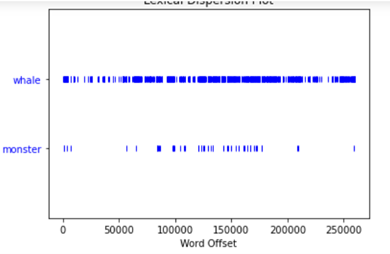
Remember that Jupyter notebooks can handle images, hence plots and graphs will be shown right in the notebook, after the command.
- text1.dispersion_plot([‘whale’, ‘monster’])
- text1.count(‘whale’)
- this command counts the requested word (or string) and is case sensitive – so searching for Whale or whale DOES make a difference.
As the count command is case sensitive, it is important to find a way to lower all words first and then count them accordingly. See below a new list made of lowered words. We can call the new list text1_tokens = []
- text1_tokens = []
- for word in text1:
- if word.isalpha():
- text1_tokens.append(word.lower())
- if word.isalpha():
It is now possible to quickly check the new list by using the following command.
- text1_tokens[:10]
The next step would be to count again; this time the result will be made of ‘whale’ + ‘Whale’ + any other combination of the word whale (i.e. ‘WhaLE’).
- text1_tokens.count(‘whale’)
Further to the above, it is possible to calculate the text’s lexical density. Lexical density represents the number of unique (or distinct) words over the total number of words. How to calculate it: len(set(list)/len(list) the function ‘set’ returns a list containing only distinct words. To exemplify:
- numbers = [1, 3, 2, 5, 2, 1, 4, 3, 1]
- set(numbers)
The output should look like the following: {1, 2, 3, 4, 5}
Let’s use this on text 1 now. The first step requires to check the unique words in the newly created ‘lowered list’. Then, the next command asks the computer to spit out only the number of unique words, and not to show the full list. Finally, it is possible to compute the ratio of unique words over total of words.
- set(text1_tokens)
- len(set(text1_tokens))
- len(set(text1_tokens)) / len(text1_tokens)
Let’s slice it now and create a list of the first 10,000 words. This allows to compare, for example, the ratio of text1 to the ratio of text2. Remember, it is very dangerous to draw conclusions based on such a simplified comparison exercise. The latter should be taken as a starting point to generate questions and provide an insightful base to work on more a complex text analysis instead.
- t1_slice = text1_tokens[:10000]
- len(t1_slice)
- len(set(t1_slice))/10000
- t2 = [word.lower() for word in text2 if word.isalpha()]
- t2_slice = t2[:10000]
- len(set(t2_slice))/10000

This entry is licensed under a Creative Commons Attribution-NonCommercial-ShareAlike 4.0 International license.
Pingback: Praxis assignment: how to ‘read’ a book without reading it | Introduction to Digital Humanities Fall 2022